I understand you.
When we start something new, we use to get so excited that we begin to google search a lot of random stuff about that thing. And it becomes almost inevitable not to get lost on the endless sea of information available on the internet. But by putting some effort, we are able to filter what is important to know based on our current level.
On this set of posts, you will be given precious information about three python libraries that you should definitely look up:
- Pandas
- NumPy
- Matplotlib
You probably already heard a thing or two about any of these. But if you didn't pay attention before - because maybe you thought they were not worth it - this is your chance to redeem yourself.
To better illustrate the next topics, consider the following dataset for demonstration purposes:
| PurchaseDate | Region | State | Seller | Item | Units | UnitPrice | |
|---|---|---|---|---|---|---|---|
| 0 | 10-Jun-2020 | Northeast | Bahia | Tobias | Stove | 62 | 400.99 |
| 1 | 11-Jun-2020 | Southeast | São Paulo | Nadia | Fridge | 29 | 100.99 |
| 2 | 3-Aug-2020 | Northeast | Ceará | Carlos | Stove | 55 | 1200.49 |
| 3 | 22-Aug-2020 | Northeast | Bahia | Pedro | Fridge | 81 | 1900.99 |
| 4 | 26-Aug-2020 | Midwest | Goiás | Tania | Blender | 42 | 2300.95 |
| 5 | 10-Sep-2020 | Northeast | Sergipe | Tobias | Carpet | 35 | 400.99 |
| 6 | 12-Sep-2020 | North | Pará | Carlos | Carpet | 3 | 2750.00 |
| 7 | 7-Oct-2020 | Northeast | Sergipe | Nadia | Blender | 2 | 1250.00 |
| 8 | 15-Oct-2020 | North | Amazonas | Pedro | Stove | 7 | 1000.29 |
| 9 | 27-Nov-2020 | Southeast | São Paulo | Nadia | Fridge | 16 | 1500.99 |
| 10 | 13-Dec-2020 | South | Paraná | Tania | Blender | 76 | 1450.99 |
file: order_data.csv
On this first post, we'll start with Pandas. And if you want to check on some specific functionality, I will leave you the table below so you can also go straight to the point.
| Load and Transform | Visualize | Locate | Summarize |
|---|---|---|---|
| read_csv | head | loc | describe |
| read_excel | tail | iloc | info |
| sort_values | shape | duplicated | sum |
| set_index | index | query | count |
| reset_index | columns | df['col'] | min |
| drop | dtypes | df.your_col | max |
| copy | isnull | --- | mean |
| --- | values | --- | median |
| --- | --- | --- | corr |
Pandas
 image by Eric Baccega
Pandas is a very powerful python library widely used by data scientists and/or analysts for both manipulating and analysing data. It also works well with many other python modules, and its main advantage is having an intuitive and practical usability without compromising its functionality.
For convenience, pandas use to be loaded into the project with the allias pd, as shown below:
import pandas as pd
It is useful so we can just use this short allias instead of typing the whole package name every time we want to use a pandas function. This library also allows us to create two type of structures that make the manipulating easier: Series and Dataframes.
Series
According to pandas official documentation, a series is a one-dimensional ndarray (an array that belongs to the NumPy class ndarray) with axis labels.
Omg, this...
Better saying, a pandas series is nothing but an unidimensional array (having a unique dimension) which can store any sort of data with labels or indexes as the axis. In short, it is like a column of a dataframe. Let's see how to create a series in pandas and how to identify its structure. The following code can be replicated in your jupyter notebook:
# imports
In [1]: import pandas as pd

# creates a series to store people names
In [2]: names = pd.Series(['Carlos', 'Sara', 'Louise', 'James'])

In [3]: names
Out[3]: 0   Carlos
        1     Sara
        2   Louise
        3    James
        dtype: object
Note that, as indexation in python begins with 0, the index range of the series created goes from 0 to n-1, where n is the number of elements on your series. This is a very important thing to remember, and which might cause a lot of malfunctioning on your codes if you mess that up.
We can also see that, as I haven't specified any index range for my series, pandas automaticatly insert the standard indexation. However, if I want a different label for my axis, I can specify that when creating the object. See how it looks:
# creates a series to store animals species
In [2]: animals = pd.Series(['Dog', 'Elephant', 'Fox', 'Eagle'],
                            index=['A', 'B', 'C', 'D'])

In [3]: animals
Out[3]: A        Dog
        B   Elephant
        C        Fox
        D      Eagle
        dtype: object
These are, in fact, very simple examples. But they might help you having an ideia of what a series look like.
Dataframes
Differently from a series, a pandas dataframe is a two-dimensional tabular structure where data is labeled by its own combination of column and row. This structure is size-mutable and potentially heterogeneous. That is, we can easily create a dataframe with two columns and two rows, and then add new columns and rows for this same object. And we can store different types of data on the same dataframe, which can be very convinient in many situations.
Let's see how it works on the jupyter notebook:
# imports
In [1]: import pandas as pd

# creates a dataframe to store people names, ages, and heights
In [2]: names = pd.DataFrame([['Carlos', 27, 1.78], ['Sara', 12, 1.35],
                              ['Louise', 35, 1.62], ['James', 18, 1.87]],
                              columns=['name', 'age', 'height'],
                              index=['i', 'ii','iii', 'iv'])

In [3]: names
Out[3]:      name   age   height
        i  Carlos    27     1.78
       ii    Sara    12     1.35
      iii  Louise    35     1.62
       iv   James    18     1.87
Could you notice how they differ? Now we have a table storing a set of information that we can either access by the index - returning all the information in a the row - or by the combination of index and columns - returning a single desired value.
And if we just want to go on regular indexing, we only need to remove the index attribute from the function.
See the official documentation for more information.
Just so to remind you, all the operations from now on will take into consideration the dataset we defiined on the very beginning of this post. Also, see that you will face many abbreviations and acronyms on your way through the data science world. I will provide you a cheatsheet on later posts.
Now, let us finally see what pandas can bring us!
Loading data
Pandas has many functions to load data into your project. You can mine data from a csv - a text file - or an excel spreadsheet, for instance. But it is also possible to get information from SQL and HTML tables, SQL query, JSON strings, Google BigQuery, Stata .dta files, and so on. See here all the options pandas offers.
Here are two frequently used functions:
pd.read_csv
For comma-separated text files.
# locate and indicate your file path
df = pd.read_csv('C:\...\order_data.csv')
pd.read_excel
For excel files.
# locate and indicate your file path
# you can also indicate the sheet name if there are more than one
df = pd.read_csv('C:\...\your_file_here.xlsx',
                      sheet_name='sheet_name_here')
Transforming data
Sometimes we only need to perform some basic transformations on our DataFrame and that's where this functions come in handy.
df.sort_values
Sort DataFrame by the values of chosen column or columns. It is possible to sort twice if you pass more than one column as parameter. You can also choose the direction of your sorting by assigning ascending as True or False.
See the documentation.
# sorts in ascending order by the column 'Seller'
df.sort_values(by='Seller', ascending=True)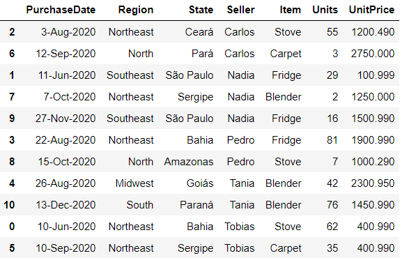
df.set_index
Set an existing DataFrame column as the index. You can either use it to replace the original index or to expand it.
See the documentation.
# using append=True to expand the index
# column 'Seller' is picked
df.set_index('Seller', append=True)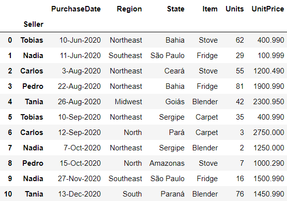
df.reset_index
Reset the index of a DataFrame, using the default one instead. Default indexation in python begin with 0. You can either drop the current index or insert it as a column into the DataFrame.
See the documentation
# drop=False keeps the current index as a column
df.reset_index(drop=False)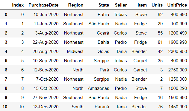
df.drop
Remove rows or columns by specifying row index or column name to drop.
For axis=0, the function searchs through the DataFrame indexes.
For axis=1, it searchs through its columns.
See the documentation
# removes PurchaseDate from the columns
df.drop('PurchaseDate', axis=1)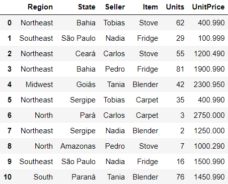
df.copy
Make a copy of the object's indices and data. If you set deep=True, none of the modifications on the original object will reflect on the copy. However, setting deep=False makes a shadow copy, and any modification on either the original or the shadow object will reflect on each other.
See the documentation
# creates a copy df
# deep=True is the default parameter
df_2 = df.copy()
print(df_2)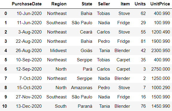
Visualizing data
df.head
Return the first n rows. If n is not specified, it returns the first 5 rows as default. It is aso possible to return everything except the last n rows by passing a negative parameter for n.
See the documentation
# returns the first 3 rows
df.head(3)
df.tail
Return the last n rows. If n is not specified, it returns the last 5 rows as default. It is aso possible to return everything except the first n rows by passing a negative parameter for n.
See the documentation
# returns everything except the first 6 rows
df.tail(-6)
df.shape
Return a tuple representing the dimensionality of the DataFrame. The first element represents the total number of rows, and the second element is the total number of columns.
See the documentation
# returns the DataFrame dimensionality
df.shape
df.index
Return the index (row labels) of the DataFrame. If the object index is the default indexation, it will return a RangeIndex object with start, stop, and step parameters.
See the documentation
# returns rows labels
df.index
df.columns
Return a list of the columns labels of the DataFrame.
See the documentation
# returns columns labels
df.columns
df.dtypes
It returns a Series with the data type of each column. If there are columns with mixed types, they'll be stored with the object dtype.
See the documentation
# returns the data type of each column
df.dtypes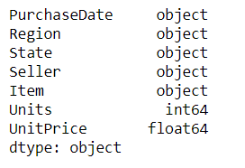
df.isnull
Used to detect missing values. As a reuslt, it returns booleans shaped as the object passed as parameter.
See the documentation
# detects missing values and returns as booleans
df.isnull()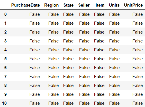
df.values
Return an array-like representation of the DataFrame. This property takes all the values of the object and returns each row as a list of values stored into a Numpy array.
See the documentation
# returns the df values as lists into a numpy array
df.values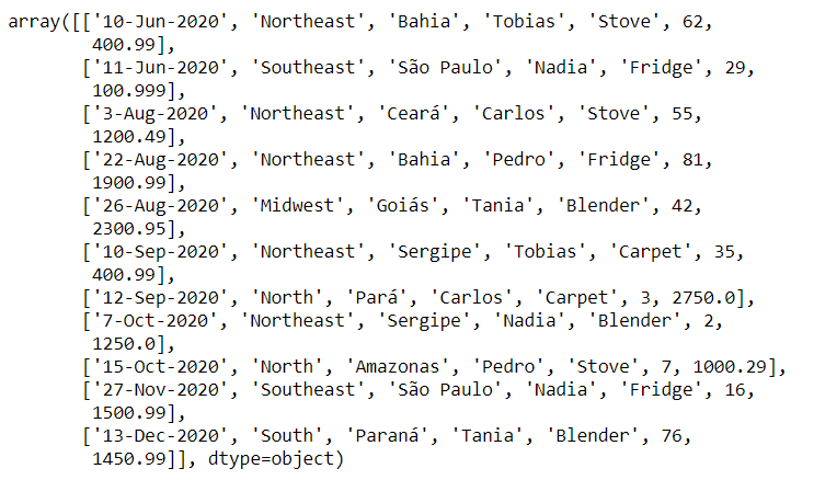
Locating data
df.loc
Access a group of rows and colums by its labels. You can use this property to either access a unique item, an entire row, or any sort of slicing of rows throughout a column or a set of columns passed as input.
See the documentation for all the input possibilities.
# access all rows stopping on label 3 of the columns Seller and Item
df.loc[:3, ['Seller', 'Item']]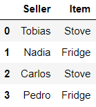
df.iloc
It is an integer position based to locate and access itens of a DataFrame. It returns all the information about a specific row.
See the documentation
# selects the indexed row 2 of the DataFrame
df.iloc[2]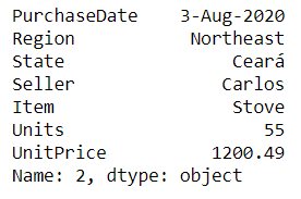
df.duplicated
Return a boolean Serie pointing the existence of duplicated rows. If no subset of columns is passed, this function will look for duplicated itens considering they are only equal if the entire rows match. You can also set the parameter keep as {'first', 'last', False} to indicate wheter you want to mark all duplicates except the first or last one as True, or if you'd like to mark all of them as True.
See the documentation
# check if there are duplicated rows when considering Seller and Item only
df.duplicated(['Seller', 'Item'])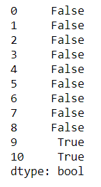
df.query
Query the columns of a DataFrame and return where the passed expression is True.
See the documentation
# queries all the values and returns where Seller is Carlos
df.query("Seller == 'Carlos'")
df['col']
This is on of the most common and simple ways to locate all the values on a entire column of a DataFrame. All you have to do is passing the columns names into the braces.
# returns all the values into the column UnitPrice
df['UnitPrice']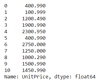
df.your_col
For a similar result as the previous locating method, you can also call the columns name as it is an attribute of the DataFrame.
# returns all the values into the column UnitPrice
df.UnitPrice
Summarizing data
df.describe
Generate a decriptive statistics table. It includes measures such as mean, median, range, standard deviation, and more.
See the documentation
# descriptive statistics with costumized percentiles
df.describe(percentiles=[0.2, 0.5, 0.8])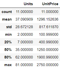
df.info
Print a summary of the DataFrame. This summary includes dtypes, columns, and non-null values.
See the documentation
# prints summary info
df.info()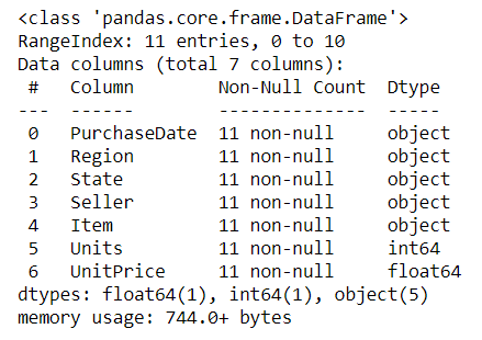
df.sum
Return the sum of the values. You can access a column first to have the results for that specific column.
See the documentation
# returns the sum for the column Units
df.Units.sum()
df.count
Count the cells with non-NA values for each row or column. NA values here are considered to be any None, NaN, NaT and numpy.inf values.
See the documentation
# counts non-null cells for each column
df.count()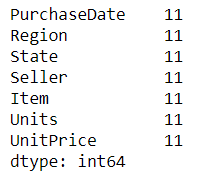
df.min
Return the minimum of the values over the requested axis. You can either request for the minimum value of some row by passing axis=0 or pass axis=1 for the minimum over a column.
See the documentation
# minimum values over the columns
df.min()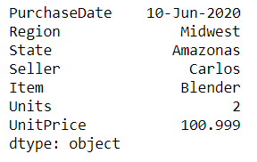
df.max
Return the maximum of the values over the requested axis.
See the documentation
# maximum value over the column UnitPrice
df.UnitPrice.max()
df.mean
Return the mean of the values over the requested axis.
See the documentation
# mean value over the column UnitPrice
df.UnitPrice.mean()
df.median
Return the median of the values over the requested axis.
See the documentation
# median value over the column UnitPrice
df.UnitPrice.median()
df.corr
Compute pairwise correlations of the DataFrame columns. It's very usefull to understand the correlation between two variables at a glance. A positive correlations indicates that the two variables varies on the same direction, while a negative correlation indicates that the two variables varies on opposite direction. On the other hand, a correlation of 0 indicates no real relationship between the variables.
See the documentation
# chacking for existing correlation between numeric variables
df.corr()
Summary
We covered up many useful functions of the Pandas python package. These are just a lightly demonstration on how this package can be used when working with data. For the intent of this post, the chosen example were pretty simple; but when we are working with large sets of data, or creating machine learning models, they are undoubtedly life savers.
Don't feel confortable with these simple examples, see the documentation to have a better understanding on everything you are able to do with them, and try if for youself on your own dataset. You'll see how easier it will become once you give it a try and compare the results by yourself!
